Getting Started
This page is intended to introduce enough theory and practical advice for a user to set up a simple shape optimization using DVGeometry.
Let’s say we want to do a structural shape optimization where we want to minimize the weight of a cylindrical pressure vessel. First, we need to generate a pointset representing the cylinder. Next, we’ll need to set up a geometric parameterization. Finally, we can perturb the geometry like an optimizer would and see the effect on the baseline cylinder shape.
Generating baseline geometry
Pointsets are collections of three-dimensional points corresponding to some geometric object.
Pointsets may represent lines, curves, triangulated meshes, quadrilateral structured meshes, or any other geometric discretization.
The pyGeo package manages all geometric parameterization in terms of pointsets.
pyGeo pointsets are always numpy arrays of dimension \(N_{\text{points}} \times 3\).
Shape optimization begins with a baseline geometry. To keep things simple, we’ll start with a cylinder centered on the point (0.5, 0.0, 0.0) extending 1.0 units along the z-axis, with a radius of 0.5. The image below shows a simple pointset on the edge of the cylinder, along with a cylinder surface for reference.
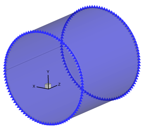
This pointset was generated using the following code snippet:
# External modules
import matplotlib.pyplot as plt
import numpy as np

# First party modules
from pygeo import DVGeometry

# create a pointset. pointsets are of shape npts by 3 (the second dim is xyz coordinate)
# we'll generate a cylinder in parametric coordinates
# the circular portion is in the x-y plane
# the depth is along the z axis
t = np.linspace(0, 2 * np.pi, 100)
Xpt = np.zeros([200, 3])
Xpt[:100, 0] = 0.5 * np.cos(t) + 0.5
Xpt[:100, 1] = 0.5 * np.sin(t)
Xpt[:100, 2] = 0.0
Xpt[100:, 0] = 0.5 * np.cos(t) + 0.5
Xpt[100:, 1] = 0.5 * np.sin(t)
Xpt[100:, 2] = 1.0
Creating an FFD volume
We will use the free-form deformation (FFD) approach to parameterize the geometry by creating a DVGeometry object.
The FFD method details are fully described in the paper, but for now it suffices to understand FFD qualitatively. First, the user creates an FFD volume, defined by a structured grid of control points. FFD volumes can be of arbitrary shape, but they tend to be rectangular or prismatic in form. They must completely enclose the pointsets to be added. Next, a pointset is embedded in the FFD volume. Finally, the control points defining the FFD volume can be moved in space.
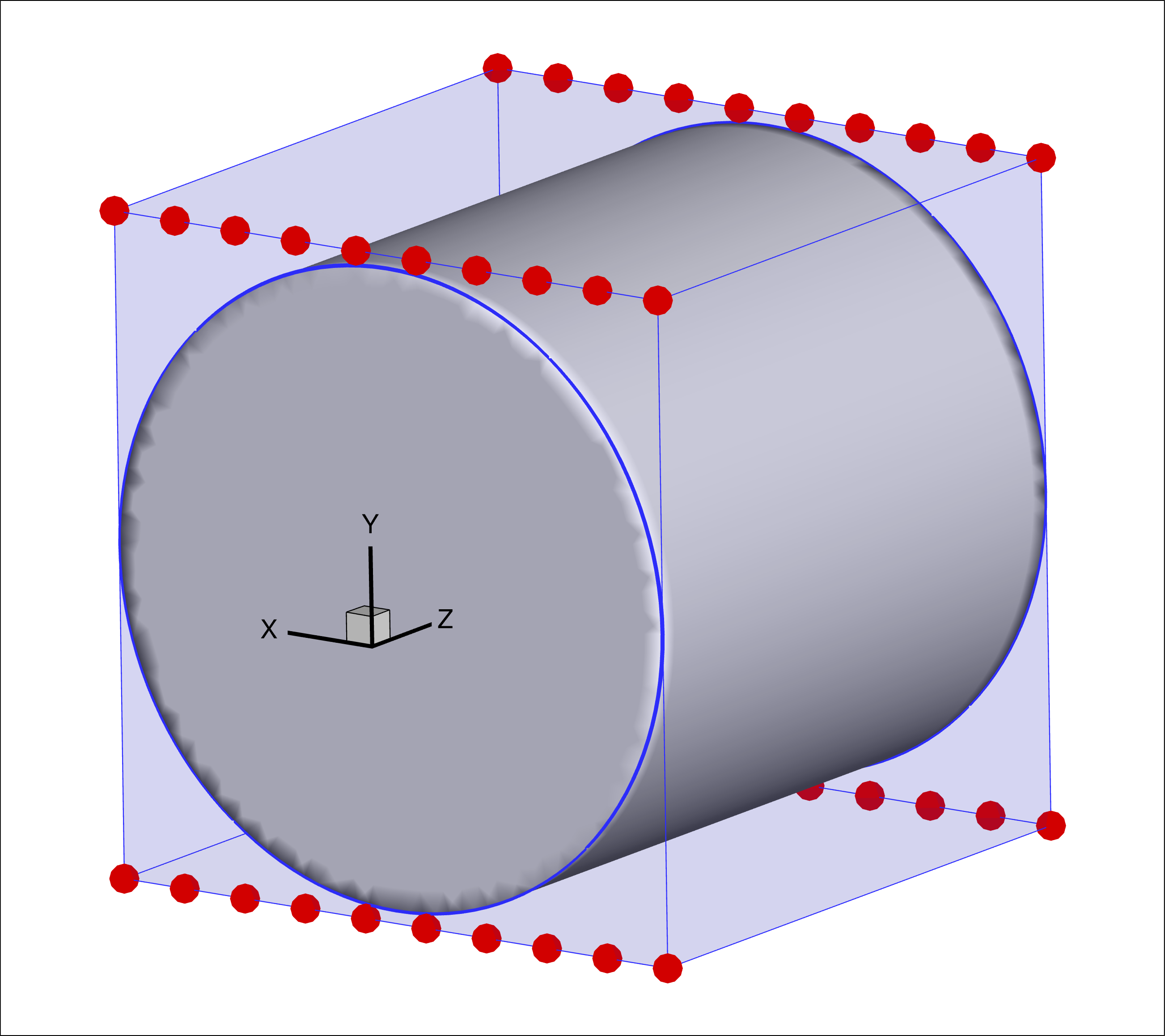
As the control points move, they stretch and twist the FFD volume as if it were a block of jelly. The points embedded in the volume move in a consistent way. The image below shows the cylinder we made embedded in a cube-shaped FFD volume. The FFD control points are depicted with the large red dots and the embedding volume is the blue shaded region.
Note
The FFD embedding volume is not necessarily coincident with the grid defined by the control points.
For example, they are coincident here (both are the region shaded in blue) but will diverge after the deformation later.
The embedded volume and FFD control points can be viewed in Tecplot using the output from writeTecplot.
pyGeo expects the FFD volume to defined in the Plot3D file format.
Points must be defined in a complete, ordered 3D grid.
The structured grid axes are typically referred to as i, j, and k axes because they do not necessarily align with the x, y, and z spatial axes.
There must be at least 2 points in each dimension.
For 3D aerodynamic shape problems where the pointset is a surface, we usually leave one dimension of length 2 and it serves as the primary perturbation direction (e.g. up and down for an airfoil design problem). The other two directions (generally streamwise and spanwise) should have more points. Airfoil design problems may have just two points in the spanwise direction (as pictured here).
The following script creates the DVGeometry object and generates the pictured cube-shaped FFD volume.
Depending on the user’s skill it may be possible to create FFD volumes which conform more closely to the pointset.
For a simple wing FFD, createFittedWingFFD can be used to generate an FFD volume that is closely fitted to a given wing geometry.
All other things being equal, a fairly tight-fitting FFD volume is better, but there can be quite a bit of margin and optimization will still work.
# External modules
import numpy as np

nffd = 10
FFDbox = np.zeros((nffd, 2, 2, 3))
xslice = np.zeros(nffd)
yupper = np.zeros(nffd)
ylower = np.zeros(nffd)

xmargin = 0.001
ymargin = 0.02
yu = 0.5
yl = -0.5

# construct the i-j (x-y) plane grid of control points 10 x 2
# we'll copy this along the k (z) axis later to make a cube
for i in range(nffd):
    xtemp = i * 1.0 / (nffd - 1.0)
    xslice[i] = -1.0 * xmargin + (1 + 2.0 * xmargin) * xtemp
    yupper[i] = yu + ymargin
    ylower[i] = yl - ymargin

# create the FFD box topology
# 1st dim = plot3d i dimension
# 2nd = plot3d j dimension
# 3rd = plot3d k dimension
# 4th = xyz coordinate dimension
# the result is a three-axis tensor of points in R3
FFDbox[:, 0, 0, 0] = xslice[:].copy()
FFDbox[:, 1, 0, 0] = xslice[:].copy()
# Y
# lower
FFDbox[:, 0, 0, 1] = ylower[:].copy()
# upper
FFDbox[:, 1, 0, 1] = yupper[:].copy()
# copy
FFDbox[:, :, 1, :] = FFDbox[:, :, 0, :].copy()
# Z
FFDbox[:, :, 0, 2] = 0.0
# Z
FFDbox[:, :, 1, 2] = 1.0

# write the result to disk in plot3d format
# the i dimension is on the rows
# j and k are on newlines
# k changes slower than j
# xyz changes slowest of all
f = open("ffdbox.xyz", "w")
f.write("1\n")
# header row with block topology n x 2 x 2
f.write(str(nffd) + " 2 2\n")
for ell in range(3):
    for k in range(2):
        for j in range(2):
            for i in range(nffd):
                f.write("%.15f " % (FFDbox[i, j, k, ell]))
            f.write("\n")
f.close()
Once we have an FFD volume file, we can finally create the actual DVGeometry object that will handle everything.
# The Plot3D file ffdbox.xyz contains the coordinates of the free-form deformation (FFD)volume
# we will be using for this problem. It's a cube with sides of length 1 centered on (0, 0,0.5).
# The "i" direction of the cube consists of 10 points along the x axis
# The "j" direction of the cube is 2 points up and down (y axis direction)
# The "k" direction of the cube is 2 points into the page (z axis direction)
FFDfile = "ffdbox.xyz"

# initialize the DVGeometry object with the FFD file
DVGeo = DVGeometry(FFDfile)
Adding pointsets
In order to retrieve parameterized pointsets later on, the baseline pointset must first be embedded in the FFD.
This is easily accomplished using the addPointSet method.
Note that each pointset gets a name.
Pointsets (whether baseline or deformed) can be written out as a Tecplot file at any time using the writePointSet method.
# add the cylinder pointset to the FFD under the name 'cylinder'
DVGeo.addPointSet(Xpt.copy(), "cylinder")
DVGeo.writePointSet("cylinder", "pointset")
Parameterizing using local shape variables
Now that we have an FFD volume and a pointset, we need to define how we want the optimizer to change and deform the geometry. We do this by adding design variables. Local design variables allow for fine control of detailed features.
We can add a variable which allows for deforming the cylinder in the y-direction as follows:
# Now that we have pointsets added, we should parameterize the geometry.

# Adding local geometric design to make local modifications to FFD box
# This option will perturb all the control points but only the y (up-down) direction
DVGeo.addLocalDV("shape", lower=-0.5, upper=0.5, axis="y", scale=1.0)
Local design variables represent perturbations to the FFD control points in the specified direction, in absolute units.
For example, setting the array of local design variables to all zeros would produce the baseline FFD shape.
Setting one entry in the array to 0.5 would pull a single control point upward by 0.5 units, which stretches the pointset locally near that control point.
Generally, local design variables are defined in only one direction: the one requiring the finest local control. Large-scale changes to the geometry in other axes can be handled well using global design variables, to be addressed later in this section.
It is important to understand a little about how the design variables are stored internally.
For implementation reasons, the raw array of control points is not in contiguous order.
If you need to access a particular control point, you can obtain its index in the design variable array by invoking the getLocalIndex method, which returns a tensor of indices addressible in the same i, j, k layout as the FFD file you created.
The following example illustrates the use of the getLocalIndex method in order to pull one slice of FFD control point coordinates (at k=0, a.k.a z=0) in contiguous order.
We can also print out the indices and coordinates of the FFD control points, which can be helpful for debugging.
# The control points of the FFD are the same as the coordinates of the points in the input file
# but they will be in a jumbled order because of the internal spline representation of the volume.
# Let's put them in a sensible order for plotting.

# the raw array of FFD control points (size n_control_pts x 3)
FFD = DVGeo.FFD.coef

# we can use the getLocalIndex method to put the coefs in contiguous order
# the FFD block has i,j,k directions
# in this problem i is left/right, j is up down, and k is into the page (along the cyl)
# Let's extract a ring of the front-face control points in contiguous order.
# We'll add these as a pointset as well so we can visualize them.
# (Don't worry too much about the details)
FFDptset = np.concatenate(
    [
        FFD[DVGeo.getLocalIndex(0)[:, 0, 0]],
        FFD[DVGeo.getLocalIndex(0)[::-1, 1, 0]],
        FFD[DVGeo.getLocalIndex(0)[0, 0, 0]].reshape((1, 3)),
    ]
).reshape(21, 3)

# Add these control points to the FFD volume. This is only for visualization purposes in this demo.
# Under normal circumstances you don't need to worry about adding the FFD points as a pointset
DVGeo.addPointSet(FFDptset, "ffd")

# Print the indices and coordinates of the FFD points for informational purposes
print("FFD Indices:")
print(DVGeo.getLocalIndex(0)[:, 0, 0])
print("FFD Coordinates:")
print(FFD[DVGeo.getLocalIndex(0)[:, 0, 0]])

# Create tecplot output that contains the FFD control points, embedded volume, and pointset
DVGeo.writeTecplot(fileName="undeformed_embedded.dat", solutionTime=1)
Perturbing local design variables
Now that we have an FFD volume, an embedded pointset, and a set of design variables, we can perturb the geometry. The following example perturbs the local design variables and illustrates how the cylinder deforms along with the control points. You can now hopefully appreciate the physical analogy of the control points as pulling on a block of jelly.
The code snippet below illustrates a few key methods of the public API.
getValuesreturns the current design variable values as a dictionary where the keys are the DV names.setDesignVarssets the design variables to new values using an input dictionary.updaterecalculates the pointset locations given potentially updated design variable values.
The updated pointset is returned from the method.
Pointsets can also be accessed as attributes of DVGeometry as required.
Note that we are using the getLocalIndex method again to perturb the design variables symmetrically.
If we perturb a control point at \(k/z = 0\), we also perturb it by the same amount at \(k/z=1\).
Otherwise, the cylinder would become skewed front-to-back.
We are also using getLocalIndex to perturb the top and bottom points differently, and in order.
Optimizers do not really care whether the points are in contiguous order, but as a human it is much easier to comprehend when addressed this way.
Also note that the dimension of the local design variable is \(N_{\text{points}}\), not \(N_{\text{points}} \times 3\). This is because when we defined the design variable, we chose the y-axis only as the perturbation direction.
# Now let's deform the geometry.
# We want to set the front and rear control points the same so we preserve symmetry along the z axis
# and we ues the getLocalIndex function to accomplish this
lower_front_idx = DVGeo.getLocalIndex(0)[:, 0, 0]
lower_rear_idx = DVGeo.getLocalIndex(0)[:, 0, 1]
upper_front_idx = DVGeo.getLocalIndex(0)[:, 1, 0]
upper_rear_idx = DVGeo.getLocalIndex(0)[:, 1, 1]

currentDV = DVGeo.getValues()["shape"]
newDV = currentDV.copy()

# add a constant offset (upward) to the lower points, plus a linear ramp and a trigonometric local change
# this will shrink the cylinder height-wise and make it wavy
# set the front and back points the same to keep the cylindrical sections square along that axis
for idx in [lower_front_idx, lower_rear_idx]:
    const_offset = 0.3 * np.ones(10)
    local_perturb = np.cos(np.linspace(0, 4 * np.pi, 10)) / 10 + np.linspace(-0.05, 0.05, 10)
    newDV[idx] = const_offset + local_perturb

# add a constant offset (downward) to the upper points, plus a linear ramp and a trigonometric local change
# this will shrink the cylinder height-wise and make it wavy
for idx in [upper_front_idx, upper_rear_idx]:
    const_offset = -0.3 * np.ones(10)
    local_perturb = np.sin(np.linspace(0, 4 * np.pi, 10)) / 20 + np.linspace(0.05, -0.10, 10)
    newDV[idx] = const_offset + local_perturb

# we've created an array with design variable perturbations. Now set the FFD control points with them
# and update the point sets so we can see how they changed
DVGeo.setDesignVars({"shape": newDV.copy()})

Xmod = DVGeo.update("cylinder")
FFDmod = DVGeo.update("ffd")

# Create tecplot output that contains the FFD control points, embedded volume, and pointset
DVGeo.writeTecplot(fileName="deformed_embedded.dat", solutionTime=1)
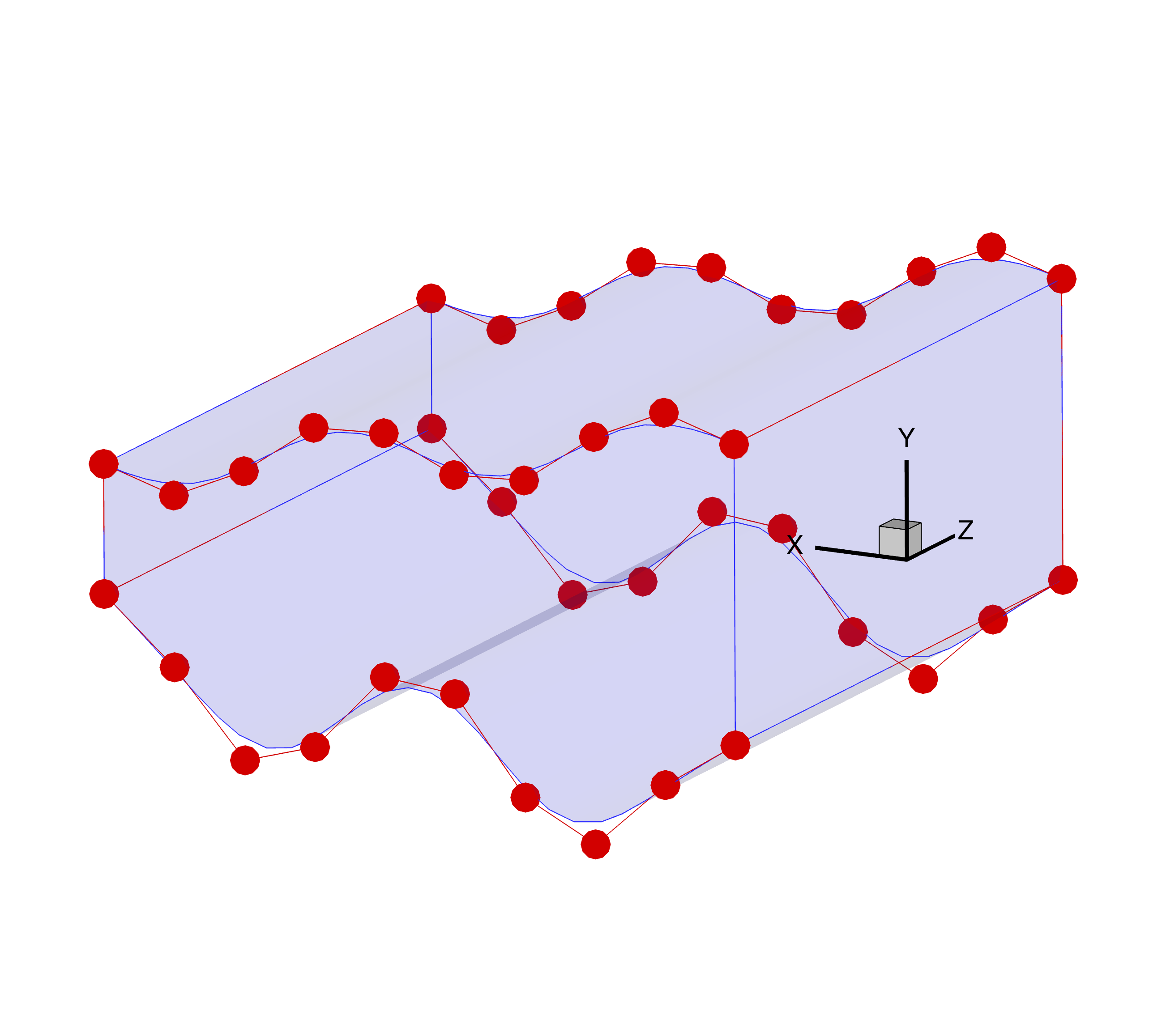
We can now see the deformed state of the FFD control points and embedding volume. Now, unlike before, the FFD embedding volume (blue lines and shaded area) is not coincident with the grid defined by the FFD control points (red circles and lines).
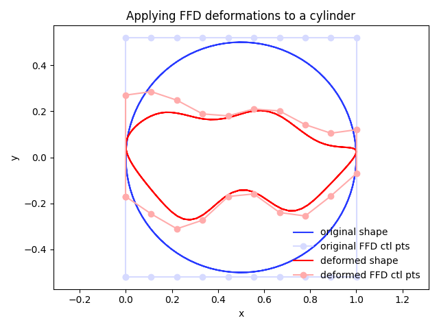
We can also compare the locations of the original and deformed FFD control points as well as the resulting shapes.
Summary
In this tutorial, you learned the basics of pyGeo’s FFD geometry parameterization capabilities.
You now know enough to set up a basic shape optimization, such as the MACH-Aero tutorial.
More advanced topics include global design variables, applying spatial constraints, and alternative parameterization options (such as ESP or OpenVSP).
The scripts excerpted for this tutorial are located at pygeo/examples/ffd_cylinder/runFFDExample.py and genFFD.py.