Advanced FFD Geometry

In the previous tutorial, we learned the basics of the free-form deformation (FFD) method of geometric parameterization. However, we limited the parameterization to perturbing the individual control points. In many applications, we will need to also allow for large-scale changes to the geometry, such as making an object longer, wider, or curved.

The purpose of this tutorial is to introduce global design variables in the DVGeometry FFD implementation. During this tutorial, we will use the Cessna 172 airplane wing as our example geometry.

_images/c172.jpg — A Cessna 172 in flight (Anna Zvereva, CC-BY)

Generating baseline geometry and FFD volume

We use the spline surfacing tool in pyGeo to generate the Cessna wing geometry from a list of airfoil sections and coordinates. A full description of the surfacing script is beyond the scope of this tutorial, but the script itself can be found at examples/c172_wing/c172.py. Using the pyiges package, one of the IGES CAD files can be converted to a triangulated (.stl) format in order to turn the wing into a pointset.

Next, we need to create an FFD volume that encloses the wing. We want to approximate the wing closely without any of the wing intersecting the box. Using our knowledge of the wing dimensions, it’s easy to create a closely-conforming FFD. The example script is located at examples/c172_wing/genFFD.py.

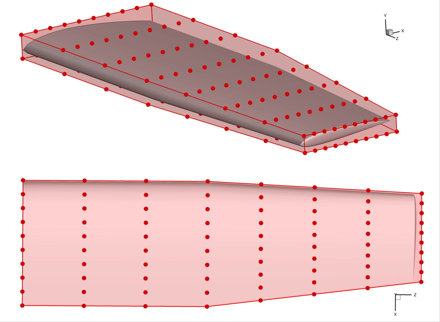
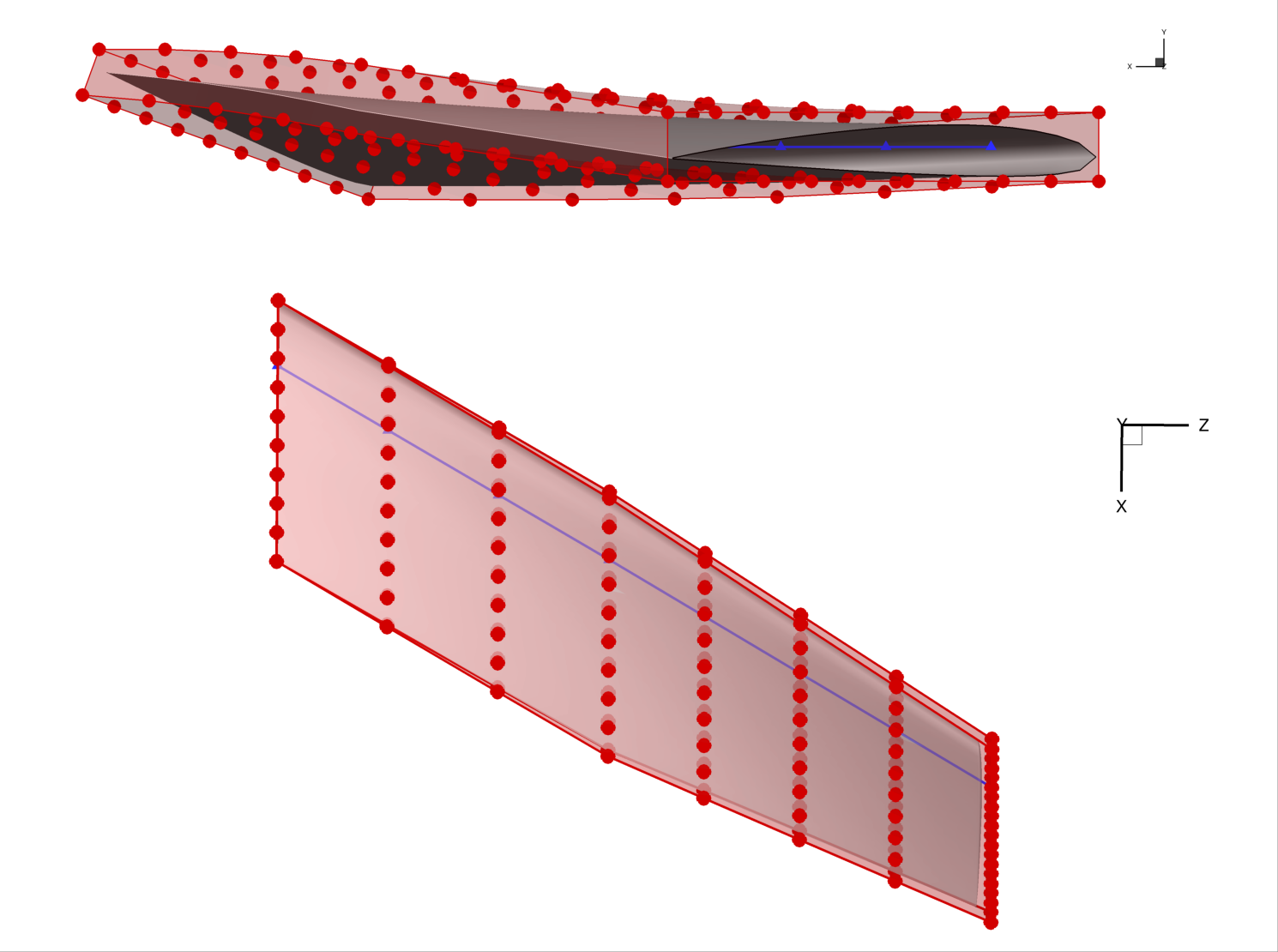
The rendering below shows the FFD volume and the point set for the wing. Note that the FFD control points are not constrained in the spanwise direction like they were in the cylinder example. We can see that the FFD volume closely approximates the wing in the top view.

Starting in the tutorial script examples/c172_wing/c172.py, we first create a DVGeometry object using the FFD file. Then, we add the wing pointset.

# External modules
import numpy as np
from stl import mesh

# First party modules
from pygeo import DVGeometry


def create_fresh_dvgeo():
    # The Plot3D file ffdbox.xyz contains the coordinates of the free-form deformation (FFD) volume
    # The "i" direction of the cube consists of 10 points along the x (streamwise) axis
    # The "j" direction of the cube is 2 points up and down (y axis direction)
    # The "k" direction of the cube is 8 along the span (z axis direction)
    FFDfile = "ffdbox.xyz"

    # initialize the DVGeometry object with the FFD file
    DVGeo = DVGeometry(FFDfile)

    stlmesh = mesh.Mesh.from_file("baseline_wing.stl")
    # create a pointset. pointsets are of shape npts by 3 (the second dim is xyz coordinate)
    # already have the wing mesh as a triangulated surface (stl file)
    # each vertex set is its own pointset, so we actually add three pointsets
    DVGeo.addPointSet(stlmesh.v0, "mesh_v0")
    DVGeo.addPointSet(stlmesh.v1, "mesh_v1")
    DVGeo.addPointSet(stlmesh.v2, "mesh_v2")
    return DVGeo, stlmesh

Adding local design variables

As in the “Getting Started” tutorial, we will first add local shape control by enabling perturbations of the individual control points in the thickness direction. In the following example, we perturb a single point in the inner portion of the wing, and then the entire upper surface at an outboard station.

# Now that we have pointsets added, we should parameterize the geometry.
# Adding local geometric design variables to make local modifications to FFD box
# This option will perturb all the control points but only the y (up-down) direction
DVGeo, stlmesh = create_fresh_dvgeo()
DVGeo.addLocalDV("shape", lower=-0.5, upper=0.5, axis="y", scale=1.0)

# Perturb some local variables and observe the effect on the surface
dvdict = DVGeo.getValues()
dvdict["shape"][DVGeo.getLocalIndex(0)[:, 1, 5]] += 0.15
dvdict["shape"][DVGeo.getLocalIndex(0)[3, 1, 1]] += 0.15
DVGeo.setDesignVars(dvdict)

# write the perturbed wing surface and ffd to output files
stlmesh.vectors[:, 0, :] = DVGeo.update("mesh_v0")
stlmesh.vectors[:, 1, :] = DVGeo.update("mesh_v1")
stlmesh.vectors[:, 2, :] = DVGeo.update("mesh_v2")
stlmesh.save("local_wing.stl")
DVGeo.writeTecplot("local_ffd.dat")

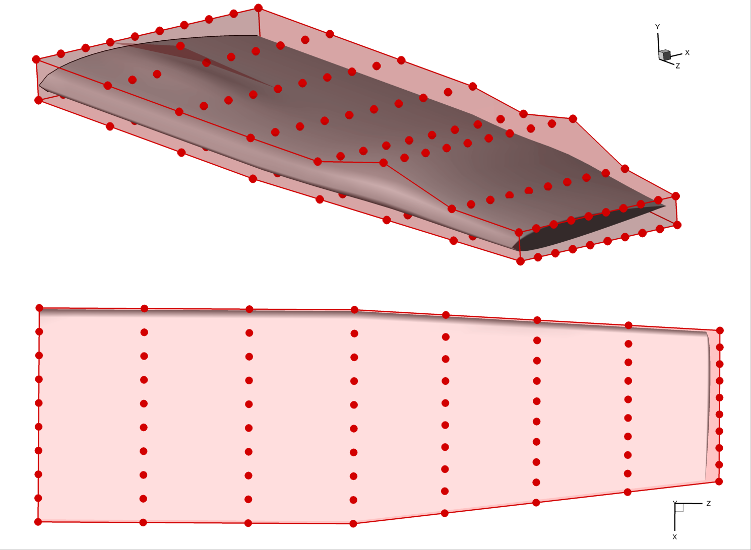
This local perturbation produces the obvious deformation in the following rendering:

Adding shape function design variables

Similar to local design variables, shape function DVs can be used to define design variables that control the local shape using a single or several control points in specified directions. The shape functions define a direction and magnitude for control points. This DV can be used to link control point movements without using linear constraints.

DVGeo, stlmesh = create_fresh_dvgeo()
# create the shape functions. to demonstrate the capability, we add 2 shape functions. each
# adds a bump to a spanwise section, and then the two neighboring spanwise sections also get
# half of the perturbation.

# this array can be access as [i,j,k] that follows the FFD volume's topology, and returns the global
# coef indices, which is what we need to set the shape
lidx = DVGeo.getLocalIndex(0)

# create the dictionaries
shape_1 = {}
shape_2 = {}

k_center = 4
i_center = 5
n_chord = lidx.shape[0]

for kk in [-1, 0, 1]:
    if kk == 0:
        k_weight = 1.0
    else:
        k_weight = 0.5

    for ii in range(n_chord):
        # compute the chord weight. we want the shape to peak at i_center
        if ii == i_center:
            i_weight = 1.0
        elif ii < i_center:
            # we are ahead of the center point
            i_weight = ii / i_center
        else:
            # we are behind the center point
            i_weight = (n_chord - ii - 1) / (n_chord - i_center - 1)

        # get the direction vectors with unit length
        dir_up = np.array([0.0, 1.0, 0.0])
        # dir down can also be defined as an upwards pointing vector. Then, the DV itself
        # getting a negative value means the surface would move down etc. For now, we define
        # the vector as its pointing down, so a positive DV value moves the surface down.
        dir_down = np.array([0.0, -1.0, 0.0])

        # scale them by the i and k weights
        dir_up *= k_weight * i_weight
        dir_down *= k_weight * i_weight

        # get this point's global index and add to the dictionary with the direction vector.
        gidx_up = lidx[ii, 1, kk + k_center]
        gidx_down = lidx[ii, 0, kk + k_center]

        shape_1[gidx_up] = dir_up
        # the lower face is perturbed with a separate dictionary
        shape_2[gidx_down] = dir_down

shapes = [shape_1, shape_2]
DVGeo.addShapeFunctionDV("shape_func", shapes)

dvdict = DVGeo.getValues()
dvdict["shape_func"] = np.array([0.3, 0.2])
DVGeo.setDesignVars(dvdict)

# write out to data files for visualization
stlmesh.vectors[:, 0, :] = DVGeo.update("mesh_v0")
stlmesh.vectors[:, 1, :] = DVGeo.update("mesh_v1")
stlmesh.vectors[:, 2, :] = DVGeo.update("mesh_v2")
stlmesh.save("shape_func_wing.stl")
DVGeo.writeTecplot("shape_func_ffd.dat")

Reference axes and global variables

Local control points are useful, but we often also want to see the effect of large-scale changes to the geometric design. For example, we may want to twist a propeller blade, or lengthen a car’s wheelbase. To do this, we need to alter many local control points at once using a mathematical transformation. We call this a global design variable.

Global design variables commonly include the following mathematical transformations:

Rotation
Linear stretching or shrinking
Translation

Rotating a point requires knowing an axis of rotation. Scaling a point requires a reference point. We can define these for the entire pointset by defining one or more reference axes. A reference axis is defined as a line or curve within the FFD volume.

You can add a reference axis to your FFD volume by using the addRefAxis method. There are two ways to define an axis. The first is to define the axis explicitly by providing a pySpline curve (using the curve keyword argument). This is the recommended approach for non-conventional FFD boxes (e.g. body-fitted sections). The second (and more commonly-used) method is to specify the direction of the reference axis in terms of the FFD dimensions (i, j, or k), along with arguments (xFraction, yFraction, zFraction) that specify the relative location of the reference axis with respect to the maximum and minimum FFD coordinates at every spanwise section along the desired dimension x, y, or z. Note that by default the reference axis node coordinates are defined using the mean of the sectional FFD points coordinates, and that the reference axis node cannot be moved outside the section plane.

The following excerpt illustrates how to create a reference axis for this Cessna 172 example. The axis is named c4 because it represents the quarter-chord line (the most useful reference point for aerodynamic analysis and design).

DVGeo, stlmesh = create_fresh_dvgeo()
# add a reference axis named 'c4' to the FFD volume
# it will go in the spanwise (k) direction and be located at the quarter chord line
nrefaxpts = DVGeo.addRefAxis("c4", xFraction=0.25, alignIndex="k")
# note that the number of reference axis points is the same as the number
# of FFD nodes in the alignIndex direction
print("Num ref axis pts: ", str(nrefaxpts), " Num spanwise FFD: 8")

# can write the ref axis geometry to a Tecplot file for visualization
DVGeo.writeRefAxes("local")

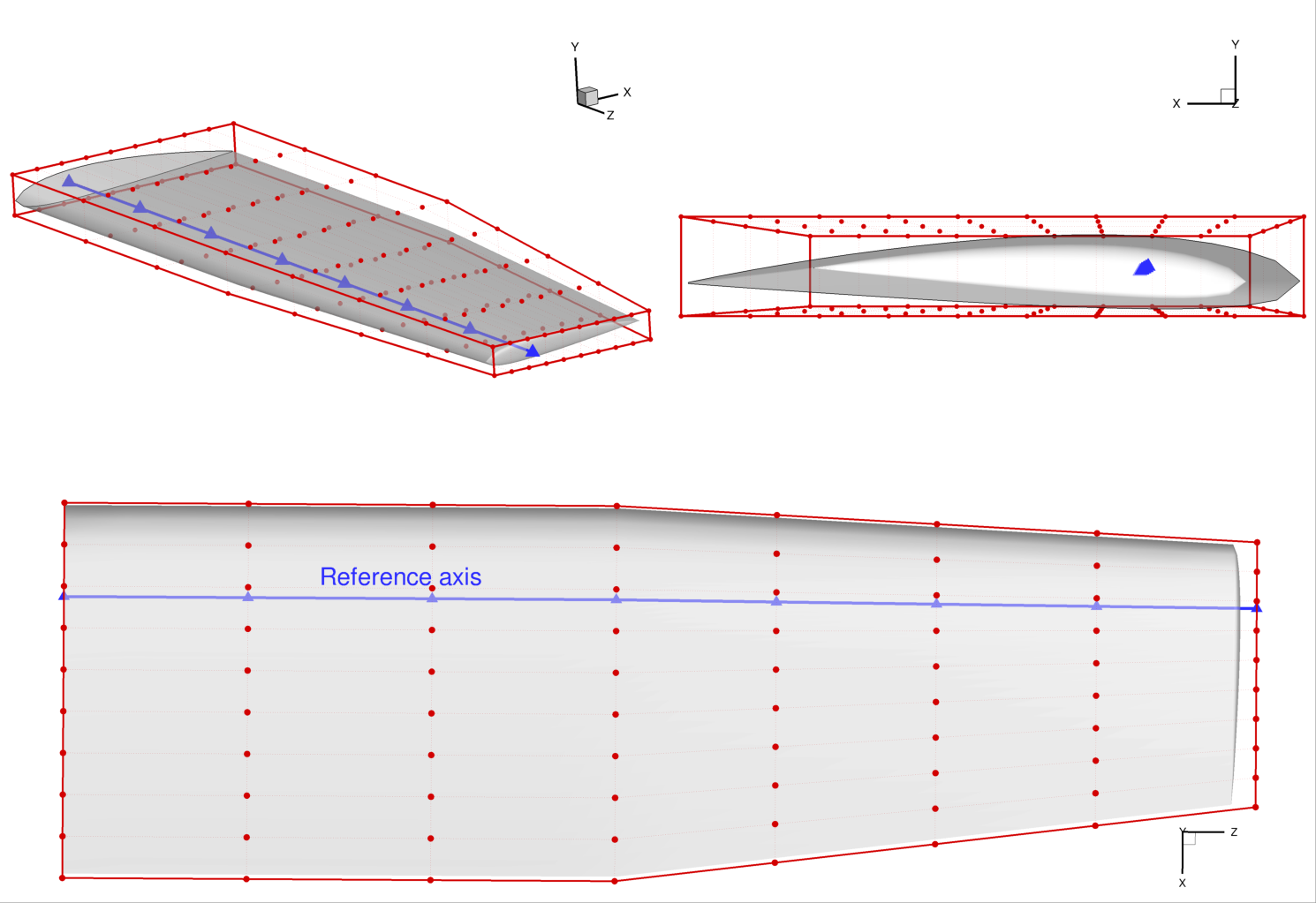
The resulting reference axis is shown in blue in this rendering:

Applying transformations

Now that we have a reference axis, we can alter the geometry globally by either:

applying transformations about the reference axis (scaling or rotation), or
moving the control points of the reference axis (translation)

Let’s start with applying a transformation, namely a twist to the wing. We need to define a function that takes in a design variable value and performs a transformation along the reference axis. The DVGeometry object has an attribute called rot_z which applies a rotation about the z-axis, and we can define a callback function to access it. It is stored as a one-dimensional spline, and it has the same number of control points as the reference axis. Indices of the rot_z control points correspond to the same location as the reference axis at that index. Other transformations include rot_x, rot_y, scale_x, and so on. This only works “in plane”, i.e. scale_ cannot move the control section and any scaling operation perpendicular to its plane will be ineffective.

The two arguments to the callback are val (the design variable value, which can be a scalar or an array), and geo which is always an instance of DVGeometry. Once we have a defined callback function, we can use the addGlobalDV method to create it as a design variable, as illustrated in the code snippet below. The parameters lower, upper, and scale are used in the optimization process (more detail can be found in the MACH-Aero tutorial but is not necessary to understand this tutorial). The optimizer can now apply a twist distribution to the wing.

# global design variable functions are callbacks that take two inputs:
# a design variable value from the optimizer, and
# the DVGeometry object itself

# the rot_z attribute defines rotations about the z axis
# along the ref axis


def twist(val, geo):
    for i in range(nrefaxpts):
        geo.rot_z["c4"].coef[i] = val[i]


# now create global design variables using the callback functions
# we just defined
DVGeo.addGlobalDV("twist", func=twist, value=np.zeros(nrefaxpts), lower=-10, upper=10, scale=0.05)

The global design variable can be perturbed just like a local design variable, as illustrated in this snippet:

# set a twist distribution from -10 to +20 degrees along the span
dvdict = DVGeo.getValues()
dvdict["twist"] = np.linspace(-10.0, 20.0, nrefaxpts)
DVGeo.setDesignVars(dvdict)
# write out the twisted wing and FFD
stlmesh.vectors[:, 0, :] = DVGeo.update("mesh_v0")
stlmesh.vectors[:, 1, :] = DVGeo.update("mesh_v1")
stlmesh.vectors[:, 2, :] = DVGeo.update("mesh_v2")
stlmesh.save("twist_wing.stl")
DVGeo.writeTecplot("twist_ffd.dat")

Applying this twist results in the geometry pictured below. The location of the reference axis (and any points located close to the reference axis) is not affected by the rotation. This is a general principle of applying transformations: the reference axis location remains invariant under the transformation.

Manipulating the reference axis

The second way to alter global geometry is by manipulating the reference axis itself. Recall that the reference axis is a spline with a number of control points. We can move these control points to produce global mesh motion just like perturbing local control points produces local motion.

We will demonstrate manipulating the reference axis by creating a sweep design variable. First, we need to define a callback function that takes in the design variable values and manipulates the axis, as shown in the snippet below. There are a few new methods to learn. extractCoef gets the array of control point values (in order) from the c4 reference axis. To sweep the wing, we apply a rotation in the x-z axis about the innermost axis point. The restoreCoef method sets the new axis position based on the manipulated points.

# sweeping back the wing requires modifying the actual
# location of the reference axis, not just defining rotations or stretching
# about the axis


def sweep(val, geo):
    # the extractCoef method gets the unperturbed ref axis control points
    C = geo.extractCoef("c4")
    C_orig = C.copy()
    # we will sweep the wing about the first point in the ref axis
    sweep_ref_pt = C_orig[0, :]

    theta = -val[0] * np.pi / 180
    rot_mtx = np.array([[np.cos(theta), 0.0, -np.sin(theta)], [0.0, 1.0, 0.0], [np.sin(theta), 0.0, np.cos(theta)]])

    # modify the control points of the ref axis
    # by applying a rotation about the first point in the x-z plane
    for i in range(nrefaxpts):
        # get the vector from each ref axis point to the wing root
        vec = C[i, :] - sweep_ref_pt
        # need to now rotate this by the sweep angle and add back the wing root loc
        C[i, :] = sweep_ref_pt + rot_mtx @ vec
    # use the restoreCoef method to put the control points back in the right place
    geo.restoreCoef(C, "c4")


DVGeo.addGlobalDV("sweep", func=sweep, value=0.0, lower=0, upper=45, scale=0.05)

Note

There is a subtle implementation detail to know. Whenever the setDesignVars method is called, the reference axis is reset back to its original values. Therefore, there’s no risk that perturbations in one optimizer iteration will stay around for the next. However, if multiple global DV callback functions manipulate the reference axis control points, only the first one will see “unperturbed” points. They will be called in the order that they are added.

Let’s apply a 30 degree sweep as well as a linear 20 degree twist. We can see how to do so in the snippet below.

# now add some sweep and change the twist a bit
dvdict = DVGeo.getValues()
dvdict["sweep"] = 30.0
dvdict["twist"] = np.linspace(0.0, 20.0, nrefaxpts)
DVGeo.setDesignVars(dvdict)

# write out the swept / twisted wing and FFD
stlmesh.vectors[:, 0, :] = DVGeo.update("mesh_v0")
stlmesh.vectors[:, 1, :] = DVGeo.update("mesh_v1")
stlmesh.vectors[:, 2, :] = DVGeo.update("mesh_v2")
stlmesh.save("sweep_wing.stl")
DVGeo.writeTecplot("sweep_ffd.dat")
DVGeo.writeRefAxes("sweep")

The results of the sweep are dramatic, as seen in the rendering.

This example illustrates an important detail; namely, that the local control points do not rotate in the x-z plane as the wing is swept back. This is because of the way the reference axis is implemented. Every local control point (the red dots) is projected onto the reference axis when the axis is created. In this case, by default, the points were projected along the x axis. Once the points are projected, they become rigidly linked to the projected point on the axis. Even if the reference axis is rotated, the rigid links do not rotate. However, the links do translate along with their reference point. Only the scale_ and rot_ operators change the rigid links. writeLinks can be used to write out these links, which can then be viewed in Tecplot.

Multiple global design variables

It is common to use several global design variables in addition to the local design variables. For example, an aircraft problem might have global design variables for wing span, taper ratio, aspect ratio, dihedral, sweep, chord distribution, and more. Each of these can be implemented through a combination of transformations and axis manipulation.

Let’s say that we want to change the chord distribution of the wing in addition to the sweep. We have to begin by writing a callback function, as follows:

# we can change the chord distribution by using the
# scale_x attribute which stretches/shrinks the pointset
# about the ref axis in the x direction


def chord(val, geo):
    for i in range(nrefaxpts):
        geo.scale_x["c4"].coef[i] = val[i]

We implement the chord distribution using the scale_x transformation which stretches points about the reference axis in the x direction. Now we need to create a global design variable and perturb the variable to produce the desired effect. Let’s also introduce a random perturbation to the local design variables to see the combined effect of sweep, twist, chord, and local deformation.

# set up a new DVGeo with all three global design vars plus local thickness
DVGeo, stlmesh = create_fresh_dvgeo()
nrefaxpts = DVGeo.addRefAxis("c4", xFraction=0.25, alignIndex="k")
DVGeo.addGlobalDV("twist", func=twist, value=np.zeros(nrefaxpts), lower=-10, upper=10, scale=0.05)
DVGeo.addGlobalDV("chord", func=chord, value=np.ones(nrefaxpts), lower=0.01, upper=2.0, scale=0.05)
DVGeo.addGlobalDV("sweep", func=sweep, value=0.0, lower=0, upper=45, scale=0.05)
DVGeo.addLocalDV("thickness", axis="y", lower=-0.5, upper=0.5)

# change everything and the kitchen sink
dvdict = DVGeo.getValues()
dvdict["twist"] = np.linspace(0.0, 20.0, nrefaxpts)
# scale_x should be set to 1 at baseline, unlike the others which perturb about 0
# the following will produce a longer wing root and shorter wing tip
dvdict["chord"] = np.linspace(1.2, 0.2, nrefaxpts)
# randomly perturbing the local variables should make a cool wavy effect
dvdict["thickness"] = np.random.uniform(-0.1, 0.1, 160)
dvdict["sweep"] = 30.0
DVGeo.setDesignVars(dvdict)

# write out to data files for visualization
stlmesh.vectors[:, 0, :] = DVGeo.update("mesh_v0")
stlmesh.vectors[:, 1, :] = DVGeo.update("mesh_v1")
stlmesh.vectors[:, 2, :] = DVGeo.update("mesh_v2")
stlmesh.save("all_wing.stl")
DVGeo.writeTecplot("all_ffd.dat")
DVGeo.writeRefAxes("all")

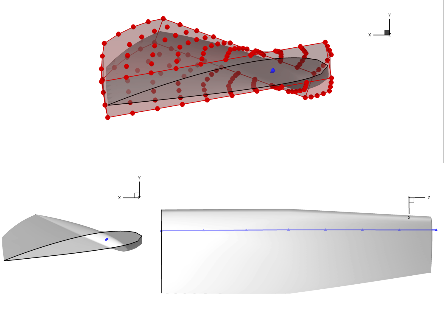
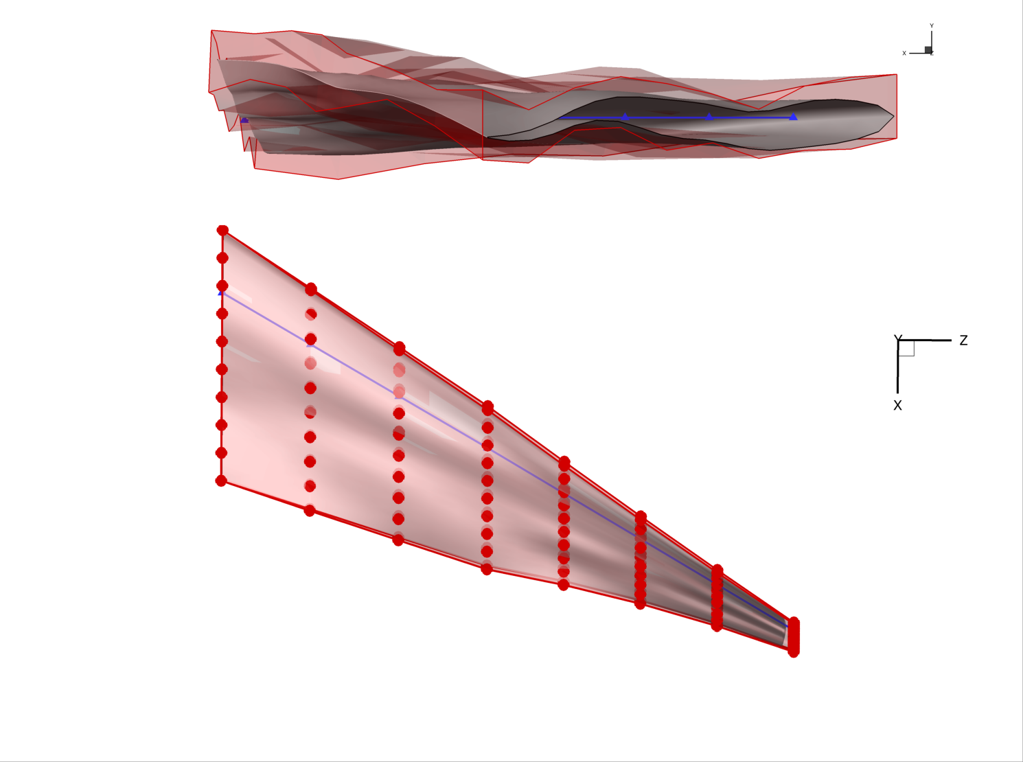
The combination of multiple global and local design variables produces the wild shape in the rendering below. Obviously this is not a suitable optimized aircraft design. However, the optimizer is free to use all of these degrees of freedom to eventually find the best possible result.

The order of operations is important when multiple global variables are used. By default, the order of operations is as follows.

There are two one-time setup steps at the beginning that happen “under the hood”:

A reference axis is created using addRefAxis.
The pointsets and FFD control points are projected onto the axis. The projected point on the axis (in parametric coordinates) is forever linked to the corresponding pointset point or FFD control point.

During each call to setDesignVars:

The reference axis control points retrieved with extractCoef are reset to the baseline values (one time! not after each callback)
Callback functions are invoked in the order they are added using addGlobalDV. The results are saved but not yet applied.

Finally, during the update method:

New reference axis projection points are computed based on the changes to the reference axis control points done by the callback functions.
Rotations are applied to the pointsets and FFD control points using the reference axis projections as the pivot point.
Depending on the choice of rotType when addRefAxis is invoked, the rot_x, rot_y, and rot_z transformations may be applied in arbitrary order. The default is z, x, y.
scale_x, scale_y, and scale_z are applied based on the vector from each point to its reference axis projection. Points on the reference axis will not change at all under either rotation or scale.
A separate scale parameter is applied which stretches all points isotropically based on their distance and direction from the reference axis projected point.
Lastly, local FFD perturbations are applied. For addLocalDV, the perturbations are applied in the Cartesian frame. For addLocalSectionDV the perturbations are applied relative to the untwisted FFD section cuts.

Summary

The FFD method can seem complicated, especially when multiple global design variables are involved. However, it is very general and has great performance, making it a good choice for general-purpose shape optimization problems.

In this tutorial, you learned how to set up global variables and make the most of FFD geometry. You now know enough to fully understand and extend more complex, FFD-based, shape optimization problems, such as those covered in the MACH-Aero tutorial.

The scripts excerpted for this tutorial are located at pygeo/examples/c172_wing/runFFDExample.py and genFFD.py.